วันนี้ได้ปรับปรุงโมเดลใหม่ พบว่าข้อมูลที่นำมาใช้พยากรณ์
มีเพียงสองวัน คือ เมื่อวาน (ไม่ก็วันศุกร์ที่แล้ว) กับ วันนี้
ก็เพียงพอที่จะพยากรณ์พรุ่งนี้ (หรือวันจันทร์หน้า) ได้แล้ว
สิ่งที่แตกต่างจากโมเดลอันก่อน นอกจากจะมี time step เป็น 2 แล้ว
ก็มีการปรับโครงสร้างโมเดล LSTM ให้มีแค่ 16 cell ทั้งหมด
มีการปรับ epoch เป็น 3 และก็มีการแก้ไข comment ในโค้ดนิดหน่อย
ก็คือเพิ่งมาสังเกตว่า dataset มีช่วงเวลาอยู่ระหว่าง
วันที่ 11 มิ.ย. 2547 จนถึงวันที่ 20 กันยายน 2567
โค้ดใหม่ที่เราทำนี้ ได้ออกแบบให้ใส่ข้อมูลได้ง่ายขึ้น
ก็คือเป็นกราฟ แล้วเลื่อนเพื่อปรับค่า high และ low เอาเอง
มันก็จะแสดงคำตอบออกมาเป็นค่าพยากรณ์ได้เลย
ไม่ว่าจะลองทำซ้ำอีกกี่ครั้ง
Train-Test Split แบบ 10:90 มันก็ดีที่สุดละ
เพราะเคยลอง 80:20, 90:10 แล้ว โมเดลไม่ได้พยากรณ์ได้ดีขึ้น
เหมือนว่ามัน Generalize ข้อมูลได้เพียงแค่นี้
Noise ต่าง ๆ ไม่สามารถพยากรณ์ได้อยู่แล้ว
เราจะแบ่งโค้ด Python ให้เพื่อน ๆ ลองเอาไปทดสอบ
โดยให้นำโค้ดไปแปะใน Google Colab
แล้วปรับ tab ให้มัน แล้วก็ค่อยรัน
ไม่จำเป็นต้องใช้ GPU, TPU แค่ CPU ก็เพียงพอแล้ว
Comment ในตัวโค้ดจะมีคำอธิบายการใช้งานอยู่นะ
ปล. ถ้าเกิดปัญหา Library มัน run ไม่ได้ จากการ import
ให้ใส่โค้ด !pip install ตามด้วย Library ที่ขาด เช่น !pip install gdown
โหลดและ Label ข้อมูล:
import pandas as pd
import numpy as np
import tensorflow as tf
import matplotlib.pyplot as plt
import gdown
from sklearn.preprocessing import MinMaxScaler
file_id = "1XXkVwG0OUQqNxWVSdz3q6IMzAnxf2dnv" # Timeframe = 1 วัน
# https://drive.google.com/file/d/1XXkVwG0OUQqNxWVSdz3q6IMzAnxf2dnv/view?usp=drive_link
# ข้อมูลได้มาจากใน Kaggle ชื่อ "XAU/USD Gold Price Historical Data (2004-2025)" ของ Novandra Anugrah
# ช่วงเวลาของข้อมูล ระหว่าง 11 มิ.ย. 2547 จนถึง 20 กันยายน 2567
csv_path = "gold_prices.csv"
gdown.download(f"https://drive.google.com/uc?id={file_id}", csv_path, quiet=False)
df = pd.read_csv(csv_path)
df['Datetime'] = pd.to_datetime(df['Date'] + ' ' + df['Time'])
df.set_index('Datetime', inplace=True)
df = df[['High', 'Low']]
def create_dataset_with_scaling(data, time_step=5):
X, Y = [], []
for i in range(len(data) - time_step):
window = data[i:i + time_step + 1]
scaler = MinMaxScaler(feature_range=(0, 1))
window_scaled = scaler.fit_transform(window)
X.append(window_scaled[:-1])
Y.append(window_scaled[-1])
return np.array(X), np.array(Y)
time_step = 2 # เวลาก่อนหน้าที่นำมาใช้พยากรณ์
X, Y = create_dataset_with_scaling(df.values, time_step)
X = np.reshape(X, (X.shape[0], X.shape[1], X.shape[2]))
โค้ด train-test split และโมเดล LSTM:
from tensorflow.keras.models import Sequential
from tensorflow.keras.layers import Input, LSTM, Dense, Dropout
train_size = int(len(X) * 0.1) # ฝึก 10% ทดสอบ 90%
X_train, X_test = X[:train_size], X[train_size:]
Y_train, Y_test = Y[:train_size], Y[train_size:]
model = Sequential([
Input(shape=(time_step, X.shape[2])),
LSTM(16, return_sequences=True),
LSTM(16, return_sequences=False),
Dense(2)
])
model.compile(optimizer='adam', loss='mean_squared_error')
model.summary()
โค้ด run ตัวโมเดล:
model.fit(X_train, Y_train, batch_size=1, epochs=3, validation_data=(X_test, Y_test))
โค้ดเช็กค่า R-Square:
from sklearn.metrics import r2_score
Y_pred = model.predict(X_test, verbose=0)
r2 = r2_score(Y_test, Y_pred)
# ค่า R-Square เป็นค่าที่อยู่ระหว่าง -1 กับ 1
# R-Square > 0 แปลว่า โมเดลพยากรณ์ได้ดีกว่าค่าเฉลี่ย
# R-Square = 0 แปลว่า โมเดลพยากรณ์ได้ไม่ต่างกับค่าเฉลี่ย
# R-Square < 0 แปลว่า โมเดลพยากรณ์ได้แย่กว่าค่าเฉลี่ย
print(f"✅ R² = {r2:.4f}")
โค้ดไว้ดูผลการพยากรณ์โดยภาพรวม:
def predict_next_day(model, data):
last_days = data[-time_step:]
scaler = MinMaxScaler(feature_range=(0, 1))
last_days_scaled = scaler.fit_transform(last_days)
last_days_scaled = last_days_scaled.reshape(1, time_step, 2)
predicted_scaled = model.predict(last_days_scaled)
predicted_actual = scaler.inverse_transform([predicted_scaled[0]])[0]
return predicted_actual
predictions_actual = []
actual_values = []
test_range = 200
start_index = len(X_test) - test_range
for i in range(start_index, len(X_test)):
scaler = MinMaxScaler(feature_range=(0, 1))
absolute_index = train_size + i
test_window = df.values[absolute_index: absolute_index + time_step + 1]
if len(test_window) < time_step + 1:
continue
scaler.fit(test_window)
pred_scaled = model.predict(X_test[i].reshape(1, time_step, 2), verbose=0)[/i]
[i] pred_actual = scaler.inverse_transform([pred_scaled[0]])[0][/i]
[i] predictions_actual.append(pred_actual)[/i]
[i] actual_values.append(test_window[-1])[/i]
[i]predictions_actual = np.array(predictions_actual)[/i]
[i]actual_values = np.array(actual_values)[/i]
[i]plt.figure(figsize=(14, 7))[/i]
[i]x = np.arange(len(actual_values))[/i]
[i]plt.fill_between(x, actual_values[:, 0], actual_values[:, 1], color='skyblue', alpha=0.4, label="Actual Range")[/i]
[i]plt.fill_between(x, predictions_actual[:, 0], predictions_actual[:, 1], color='salmon', alpha=0.4, label="Predicted Range")[/i]
[i]plt.plot(x, actual_values[:, 0], color='blue', label="Actual High", linewidth=1)[/i]
[i]plt.plot(x, actual_values[:, 1], color='blue', label="Actual Low", linewidth=1, linestyle='dotted')[/i]
[i]plt.plot(x, predictions_actual[:, 0], color='red', label="Predicted High", linewidth=1)[/i]
[i]plt.plot(x, predictions_actual[:, 1], color='red', label="Predicted Low", linewidth=1, linestyle='dotted')[/i]
[i]plt.title(f"Gold Price Range Prediction (Last {test_range} Days)")[/i]
[i]plt.xlabel("Day Index")[/i]
[i]plt.ylabel("Price")[/i]
[i]plt.legend()[/i]
[i]plt.grid(True)[/i]
[i]plt.tight_layout()[/i]
[i]plt.show()
ซึ่ง ณ ตอนนี้ โมเดลสามารถพยากรณ์ในภาพรวมจากข้อมูลตัวอย่างได้แบบนี้:
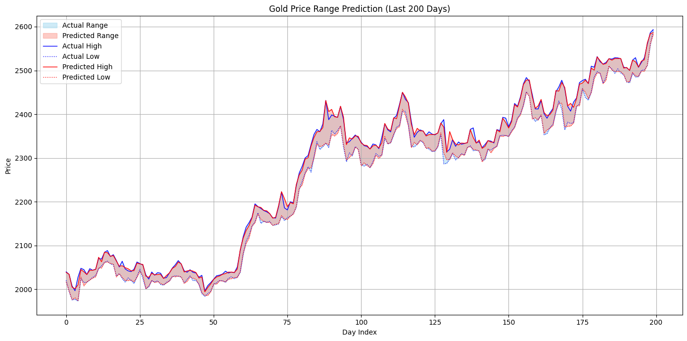

โมเดล LSTM เวอร์ชันที่ 2 ไว้พยากรณ์ high และ low ของราคาทองคำในวันพรุ่งนี้ (ค่า R² ที่ทำได้ = 0.7323)
มีเพียงสองวัน คือ เมื่อวาน (ไม่ก็วันศุกร์ที่แล้ว) กับ วันนี้
ก็เพียงพอที่จะพยากรณ์พรุ่งนี้ (หรือวันจันทร์หน้า) ได้แล้ว
สิ่งที่แตกต่างจากโมเดลอันก่อน นอกจากจะมี time step เป็น 2 แล้ว
ก็มีการปรับโครงสร้างโมเดล LSTM ให้มีแค่ 16 cell ทั้งหมด
มีการปรับ epoch เป็น 3 และก็มีการแก้ไข comment ในโค้ดนิดหน่อย
ก็คือเพิ่งมาสังเกตว่า dataset มีช่วงเวลาอยู่ระหว่าง
วันที่ 11 มิ.ย. 2547 จนถึงวันที่ 20 กันยายน 2567
โค้ดใหม่ที่เราทำนี้ ได้ออกแบบให้ใส่ข้อมูลได้ง่ายขึ้น
ก็คือเป็นกราฟ แล้วเลื่อนเพื่อปรับค่า high และ low เอาเอง
มันก็จะแสดงคำตอบออกมาเป็นค่าพยากรณ์ได้เลย
Train-Test Split แบบ 10:90 มันก็ดีที่สุดละ
เพราะเคยลอง 80:20, 90:10 แล้ว โมเดลไม่ได้พยากรณ์ได้ดีขึ้น
เหมือนว่ามัน Generalize ข้อมูลได้เพียงแค่นี้
Noise ต่าง ๆ ไม่สามารถพยากรณ์ได้อยู่แล้ว
เราจะแบ่งโค้ด Python ให้เพื่อน ๆ ลองเอาไปทดสอบ
โดยให้นำโค้ดไปแปะใน Google Colab
แล้วปรับ tab ให้มัน แล้วก็ค่อยรัน
ไม่จำเป็นต้องใช้ GPU, TPU แค่ CPU ก็เพียงพอแล้ว
Comment ในตัวโค้ดจะมีคำอธิบายการใช้งานอยู่นะ
ปล. ถ้าเกิดปัญหา Library มัน run ไม่ได้ จากการ import
ให้ใส่โค้ด !pip install ตามด้วย Library ที่ขาด เช่น !pip install gdown
โหลดและ Label ข้อมูล:
import numpy as np
import tensorflow as tf
import matplotlib.pyplot as plt
import gdown
from sklearn.preprocessing import MinMaxScaler
file_id = "1XXkVwG0OUQqNxWVSdz3q6IMzAnxf2dnv" # Timeframe = 1 วัน
# https://drive.google.com/file/d/1XXkVwG0OUQqNxWVSdz3q6IMzAnxf2dnv/view?usp=drive_link
# ข้อมูลได้มาจากใน Kaggle ชื่อ "XAU/USD Gold Price Historical Data (2004-2025)" ของ Novandra Anugrah
# ช่วงเวลาของข้อมูล ระหว่าง 11 มิ.ย. 2547 จนถึง 20 กันยายน 2567
csv_path = "gold_prices.csv"
gdown.download(f"https://drive.google.com/uc?id={file_id}", csv_path, quiet=False)
df = pd.read_csv(csv_path)
df['Datetime'] = pd.to_datetime(df['Date'] + ' ' + df['Time'])
df.set_index('Datetime', inplace=True)
df = df[['High', 'Low']]
def create_dataset_with_scaling(data, time_step=5):
X, Y = [], []
for i in range(len(data) - time_step):
window = data[i:i + time_step + 1]
scaler = MinMaxScaler(feature_range=(0, 1))
window_scaled = scaler.fit_transform(window)
X.append(window_scaled[:-1])
Y.append(window_scaled[-1])
return np.array(X), np.array(Y)
time_step = 2 # เวลาก่อนหน้าที่นำมาใช้พยากรณ์
X, Y = create_dataset_with_scaling(df.values, time_step)
X = np.reshape(X, (X.shape[0], X.shape[1], X.shape[2]))
from tensorflow.keras.layers import Input, LSTM, Dense, Dropout
train_size = int(len(X) * 0.1) # ฝึก 10% ทดสอบ 90%
X_train, X_test = X[:train_size], X[train_size:]
Y_train, Y_test = Y[:train_size], Y[train_size:]
model = Sequential([
Input(shape=(time_step, X.shape[2])),
LSTM(16, return_sequences=True),
LSTM(16, return_sequences=False),
Dense(2)
])
model.compile(optimizer='adam', loss='mean_squared_error')
model.summary()
Y_pred = model.predict(X_test, verbose=0)
r2 = r2_score(Y_test, Y_pred)
# ค่า R-Square เป็นค่าที่อยู่ระหว่าง -1 กับ 1
# R-Square > 0 แปลว่า โมเดลพยากรณ์ได้ดีกว่าค่าเฉลี่ย
# R-Square = 0 แปลว่า โมเดลพยากรณ์ได้ไม่ต่างกับค่าเฉลี่ย
# R-Square < 0 แปลว่า โมเดลพยากรณ์ได้แย่กว่าค่าเฉลี่ย
print(f"✅ R² = {r2:.4f}")
last_days = data[-time_step:]
scaler = MinMaxScaler(feature_range=(0, 1))
last_days_scaled = scaler.fit_transform(last_days)
last_days_scaled = last_days_scaled.reshape(1, time_step, 2)
predicted_scaled = model.predict(last_days_scaled)
predicted_actual = scaler.inverse_transform([predicted_scaled[0]])[0]
return predicted_actual
predictions_actual = []
actual_values = []
test_range = 200
start_index = len(X_test) - test_range
for i in range(start_index, len(X_test)):
scaler = MinMaxScaler(feature_range=(0, 1))
absolute_index = train_size + i
test_window = df.values[absolute_index: absolute_index + time_step + 1]
if len(test_window) < time_step + 1:
continue
scaler.fit(test_window)
pred_scaled = model.predict(X_test[i].reshape(1, time_step, 2), verbose=0)[/i]
[i] pred_actual = scaler.inverse_transform([pred_scaled[0]])[0][/i]
[i] predictions_actual.append(pred_actual)[/i]
[i] actual_values.append(test_window[-1])[/i]
[i]predictions_actual = np.array(predictions_actual)[/i]
[i]actual_values = np.array(actual_values)[/i]
[i]plt.figure(figsize=(14, 7))[/i]
[i]x = np.arange(len(actual_values))[/i]
[i]plt.fill_between(x, actual_values[:, 0], actual_values[:, 1], color='skyblue', alpha=0.4, label="Actual Range")[/i]
[i]plt.fill_between(x, predictions_actual[:, 0], predictions_actual[:, 1], color='salmon', alpha=0.4, label="Predicted Range")[/i]
[i]plt.plot(x, actual_values[:, 0], color='blue', label="Actual High", linewidth=1)[/i]
[i]plt.plot(x, actual_values[:, 1], color='blue', label="Actual Low", linewidth=1, linestyle='dotted')[/i]
[i]plt.plot(x, predictions_actual[:, 0], color='red', label="Predicted High", linewidth=1)[/i]
[i]plt.plot(x, predictions_actual[:, 1], color='red', label="Predicted Low", linewidth=1, linestyle='dotted')[/i]
[i]plt.title(f"Gold Price Range Prediction (Last {test_range} Days)")[/i]
[i]plt.xlabel("Day Index")[/i]
[i]plt.ylabel("Price")[/i]
[i]plt.legend()[/i]
[i]plt.grid(True)[/i]
[i]plt.tight_layout()[/i]
[i]plt.show()